Home / The math

The mathematics, explained

Each mechanism in the framework is one piece of mean-field / control theory. This page states every equation, says what each symbol means in plain language, flags the four places where a naive version is wrong, and hands you a slider to move. The sliders run the same primitives the paper verifies; they demonstrate internal consistency, never empirical proof. For empirical contact, see Tests & data.

#MechanismThe core equation
1Attention conservationcontinuity equation: $\partial_t \rho + \nabla\!\cdot J = 0$
2Belief as a drift field$J = \rho v - D\nabla\rho + \rho\, b$
3Near-decomposability & Neffvariance-ratio $N_{\mathrm{eff}} = \mathrm{Var}(x_k)/\mathrm{Var}(\bar x)$
4Criticality, Kc & the skill horizonKuramoto order $r$; $\tau^\* \propto N_{\mathrm{eff}}/K$
5Reflexivity & MFG fixed points$\rho^\* = T(\rho^\*)$, Lasry–Lions equilibrium
6Observation & assimilationEnKF update + normalized-innovation monitor
7The engine turned on AIcapture → $N_{\mathrm{eff}}$ collapse → phase flip
1 · Attention conservation

Attention is a conserved normalized measure

The first repair to "society has no conservation law." Total collective attention over a population is, to first order, a fixed budget: a panic creates no new hours in the day. What looks like belief appearing from nowhere is attention being reallocated. Write $\rho(x,t)$ for the density of attention over topics $x$. It obeys a continuity equation.

The continuity equation

$$\frac{\partial \rho}{\partial t} + \nabla\!\cdot J = s(x,t), \qquad \int \rho\,dx = 1.$$

Where: ρ is the attention density (a probability measure that integrates to 1); J is the attention flux (how attention flows between topics); s is a small source/sink term for genuine entry and exit of attention into the system. With $s\!\approx\!0$ the integral of $\rho$ is invariant: attention moves, it is not created.

This is the Fokker–Planck / Toscani "conserved normalized measure" reading. Correction 1

What the naive version got wrong: a softmax over topic scores is not a conservation law — it is a normalization applied at each instant, which is a category error. The conserved object is a probability measure transported by a continuity equation, not a softmax output. The distinction matters because only the transport reading gives you fluxes, drift, and the SVB-style 48-hour reallocation dynamics.

DEMO A · L2

Attention conservation + belief drift

Twelve topics share a fixed attention budget on a ring. A belief drift biases flow toward topic #7 (cyan). Move the drift; watch attention concentrate while the total stays pinned at exactly 1.000000.

total mass
1.000000 (the conserved quantity)
peak share
0.083 on topic #7
HHI
0.083 (concentration index)
step
0
2 · Belief as a drift field

Belief is a direction, not a stock

Why not just call belief a kind of attention? Because belief fails the sign test: you can attend maximally to what you reject. So belief is not a conserved sub-measure — it is a drift imposed on attention's transport. It enters the flux $J$, not the density $\rho$.

The flux decomposition

$$J = \underbrace{\rho\,v}_{\text{advection}} \;-\; \underbrace{D\,\nabla\rho}_{\text{diffusion}} \;+\; \underbrace{\rho\,b}_{\text{belief drift}}.$$

Where: v is a baseline advective velocity (where attention is already heading); D is a diffusion constant (attention spreads to neighbouring topics); b is the belief drift field — a direction that biases the flux. Valence (approve vs reject) rides on top of all this as a separate, non-conserved order parameter, the magnetization analogue.

Reading it: high $\rho$ with $b$ pointing inward is legitimacy; high $\rho$ with $b$ pointing outward is crisis — a bank at 48-hour run intensity. Demo A above is exactly this equation with $v=0$, a small $D$, and a tunable $b$ toward one topic.

§ Honest: the advective and belief terms are an exact directed transport; the diffusion term conserves only the integral of $\rho$, not a per-unit ledger. The continuity equation is a statement about the total, not a receipt for each unit of attention.

3 · Near-decomposability & the effective sample size

The statistical unit is the block, not the person

The second repair, to "agents are correlated, so the law of large numbers fails." Society is nearly decomposable (Herbert Simon): dense interaction inside a community, sparse between. So you do not average over people — you average over blocks, and the effective number of independent units is $N_{\mathrm{eff}}$, which can be far below both the population and the block count $K$.

The effective number of independent blocks

$$N_{\mathrm{eff}} \;=\; \frac{\operatorname{Var}_t\!\big(x_k(t)\big)}{\operatorname{Var}_t\!\big(\bar x(t)\big)} \quad\text{(macro variance-ratio, the canonical estimator).}$$

Where: $x_k(t)$ is the activity of block $k$ over time, $\bar x(t)=\frac1K\sum_k x_k(t)$ is the population mean. If the $K$ blocks are independent, the mean's variance is $1/K$ of a single block's, so $N_{\mathrm{eff}}\!\approx\!K$. If they synchronize, $\bar x$ swings as hard as any single block and $N_{\mathrm{eff}}\!\to\!1$: the law of large numbers has evaporated.

There is a closed-form Kish/Pearson version, $N_{\mathrm{eff}}=K/\big(1+(K-1)\bar\rho\big)$, where $\bar\rho$ is the mean cross-block correlation. Correction 2

What the naive version got wrong: estimating $\bar\rho$ from the Pearson correlation of fluctuations badly understates synchronization — in the verified E4 simulation it stays near 64 while the system collapses to 1. The macro variance-ratio is the estimator that actually tracks the collapse (61 → 1). The Kish form is shown in red on the demo precisely so you can watch it mislead.

DEMO B · L3 / L5

Block synchronization & the Neff collapse

48 coupled blocks. Raise the coupling $W$ and watch synchrony $S$ rise, the effective number of independent blocks fall toward 1, and the skill horizon $\tau^\*$ collapse. The red dotted line is the misleading Pearson estimator — note how it barely moves while the system goes critical.

synchrony S
Neff (correct)
of 48
Neff (Pearson)
 — the misleading one
skill horizon τ*
model-time
4 · Criticality, the critical coupling, and the skill horizon

Where forecasting fails — and control takes over

The collapse in Demo B is a phase transition. Past a critical coupling $K_c$ the blocks lock into a single mode; below it they are effectively independent. The same crossing controls how far ahead you can predict.

The Kuramoto order parameter and critical coupling

$$r\,e^{i\psi} = \frac1N\sum_{j=1}^{N} e^{i\theta_j}, \qquad K_c = \frac{2}{\pi\, g(0)}.$$

Where: $r\in[0,1]$ is the synchronization order parameter (0 = incoherent, 1 = fully locked); $\theta_j$ are the phases of the coupled units; $K_c$ is the critical coupling at which synchronization switches on, set by the spread $g(0)$ of natural frequencies. "World Cup" (many independent conversations) is the sub-critical phase; "Pluribus" (one locked conversation) is super-critical. They are one transition with two names.

The verified check: the simulation recovers $K_c \approx 0.969$ against a theoretical $1.0$ (3.1% error), instantiating the first-vs-second-moment machinery that the $N_{\mathrm{eff}}$ collapse rides on.

The skill horizon collapses at the transition

$$\tau^\* \;\propto\; \frac{N_{\mathrm{eff}}}{K}.$$

Where: $\tau^\*$ is the forecast skill horizon — how far ahead an ensemble forecast stays useful before perturbations diverge. As $N_{\mathrm{eff}}\to 1$ near the transition, $\tau^\*\to 0$: the system becomes unpredictable exactly when the stakes are highest. This is not a failure of compute; it is the structure. The right move is to switch the objective from predicting which branch to forecasting that a transition is near — and, only under governance, to use the same divergent susceptibility for control.
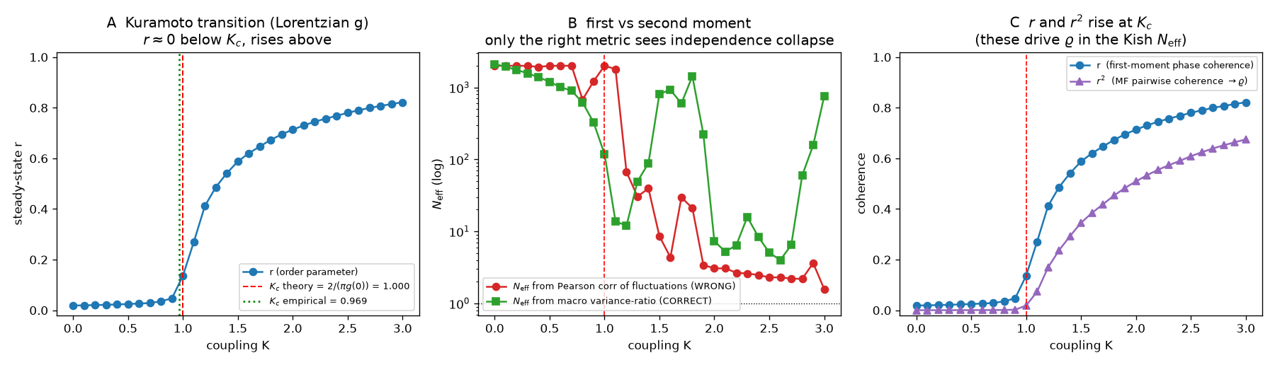
Kuramoto critical coupling: empirical K_c vs theory
The Kuramoto $K_c$ demonstration: empirical critical coupling $0.969$ vs theory $1.0$. Below $K_c$ the order parameter $r$ sits near zero (independent blocks); above it $r$ rises sharply (the locked phase) — the same transition you drive with the slider in Demo B.

§ Early-warning is valid only for slow B-tipping. Rising variance and synchrony precede bifurcation tipping — but the prosecutor's fallacy applies (a warning is not a guarantee), and noise-induced (N-) and rate-induced (R-) tipping have no warning at all. The blind spots are real and are reported as such; the empirical bifurcation-mix test (Tests) found most real cascades are sudden R-tipping shocks.

5 · Reflexivity & mean-field-game fixed points

A forecast that survives being published

The third repair, to "the forecast is an input to the system." A social prediction, once published and acted upon, changes the outcome. The resolution: only publish fixed points — predictions that remain true after everyone best-responds to them. These are the equilibria of a mean-field game.

The fixed-point condition

$$\rho^\* = T(\rho^\*),$$

Where: $T$ is the prediction–reaction map — it takes a believed distribution $\rho$, lets every agent best-respond, and returns the realized distribution. A fixed point $\rho^\*$ is a forecast that reproduces itself: publishable because it is self-consistent. This is the Lasry–Lions mean-field-game equilibrium; it pairs a backward Hamilton–Jacobi–Bellman equation (each agent optimizing) with a forward Fokker–Planck equation (the crowd it produces).

Two regimes. Correction 4 In the monotone (congestion) regime — agents avoid crowds — the fixed point is unique and the forecast is publishable. In the imitative regime — agents chase crowds — the map is bistable: a "run" fixed point and a "no-run" fixed point with an unstable threshold between them. Bistability is exactly where open-loop forecasting fails and control takes over. A unique publishable forecast exists only in the monotone regime.

DEMO C · L4

Reflexive fixed points — the bank run

The reaction map $T(f)$ for a bank run: given an expected run-fraction $f$, how many actually run? Fixed points are where $T(f)=f$. Raise the deposit guarantee $g$ to kill the run; lower the imitative coupling $c$ to expose bistability.

fixed points
equilibrium run-fraction
regime
6 · Observation & assimilation

Estimating the state, and knowing when you have left the model

The engine is a state-space system: it estimates a hidden social state, assimilates noisy observations, runs a perturbed ensemble forward, and reports its spread plus an honest skill horizon. The load-bearing piece is the self-diagnosis — a monitor that fires when reality has left the model (the "Mule" / out-of-distribution event).

The ensemble update and the misspecification monitor

$$x_a = x_f + K\big(y - Hx_f\big), \qquad z_t = \frac{y_t - H x_{f,t}}{\sqrt{S_t}}.$$

Where: $x_f$ is the forecast (prior) state, $y$ the observation, $H$ the observation operator, $K$ the Kalman gain that optimally weights prior against data, and $x_a$ the updated (posterior) estimate. The second quantity $z_t$ is the normalized innovation: the surprise of each observation in units of its own predicted standard deviation $\sqrt{S_t}$. When $|z_t|$ blows past its expected range, the model is being falsified in real time — no future information required.

What the data showed: run strictly causally on r/AskEconomics monthly activity, the filter beat climatology and was best-calibrated, but did not beat a persistence (last-value) baseline — an honest negative. The win was the monitor firing at $z=-3.33$ on a real April-2025 regime break. ▸ the full EnKF test

7 · The engine turned on AI itself

Scenario: World Cup vs Pluribus

A forward projection of the same machinery applied to AI. Capability growth and falling cost drive attention capture; cognition routes through ever-fewer model lineages; cross-human correlation rises and the effective number of independent decision-communities $N_{\mathrm{eff}}$ collapses. The same smooth-vs-critical boundary that governs every panel above decides whether psychohistory still holds. The robust output is the ordering of events, never a date.

SCENARIO · L2→L3→L5 · the Mythos Fable

Capture → Neff collapse → phase flip

This phase boundary is the same smooth-vs-critical boundary as Demo B: sub-critical = many adversarial blocks (the LLN holds, forecasting works); super-critical = Neff→1 (the recovered LLN evaporates, psychohistory fails).

Leff (model lineages)
of 50
end Neff
of K
Neff=10 crossing
skill horizon τ*

§ The OOD-shock inset shows the derived Second Foundation result: an open-loop model diverges after a regime break, while a standing detect-and-correct loop stays bounded — and lineage diversity (higher $L_{\mathrm{eff}}$, lower $\rho_{\mathrm{model}}$) partially substitutes for the central corrector. A monoculture needs the controller; diversity is partly self-healing.

Next: what happened when these mechanisms met real data ▸